Exercise 1

ENM/SDM for Podarcis muralis

Background

We already modeled the niche and distribution of the species Podarcis muralis in the lecture Running our first ENM/SDM. We, however, tried only two sets of climatic predictors for this species. Here, your task is to re-run the two ENMs from that lecture and two more ENMs using different climatic variables. In particular, you should:

1. Run 2 more ENMs.
2. Check their theoretical validity.
3. Check their statistical support.
4. Select the best ENM.
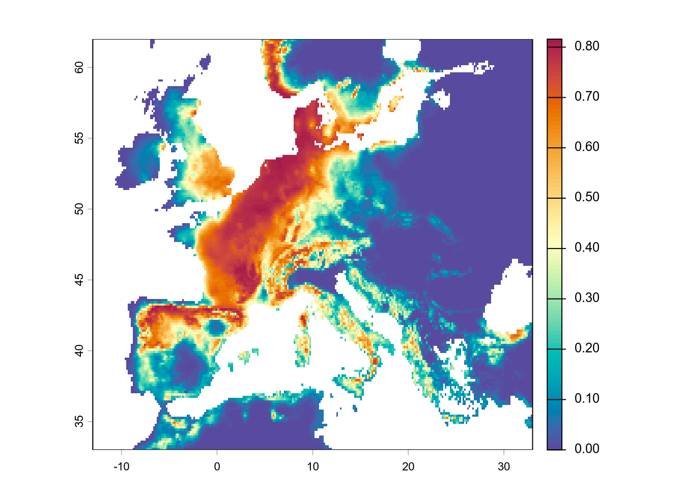
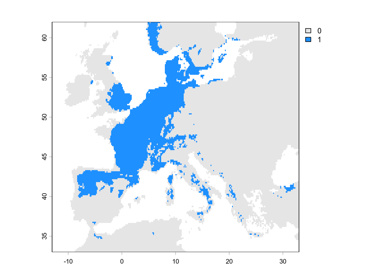
5. Use that ENM for SDM (continuous and binary).

Set-up

To set up the exercise, load all climatic layers and data for ENM/SDM.

library(terra)

# load data frame for ENM
d <- read.csv("../data/occurrences.csv")

# load climate data for SDM
ff <- list.files("../data", pattern = ".tif") # all files with .tif extension
r <- rast(file.path("..", "data", ff))
roi <- ext(-13, 33, 33, 62) # roi of Europe
r <- crop(r, roi) # crop to Europe

# ENM-1
enm_01_12 <- glm(
  occ ~ poly(wc2.1_10m_bio_1, 2, raw = TRUE) + poly(wc2.1_10m_bio_12, 2, raw = TRUE),
  data = d,
  family = "binomial"
)

# ENM-2
enm_06_14 <- glm(
  occ ~ poly(wc2.1_10m_bio_6, 2, raw = TRUE) + poly(wc2.1_10m_bio_14, 2, raw = TRUE),
  data = d,
  family = "binomial"
)

# Exercise starts from here
# ...

Solution

Run 2 more ENMs

# EMN-3 = only temperature variables
enm_01_04 <- glm(
  occ ~ poly(wc2.1_10m_bio_1, 2, raw = TRUE) + poly(wc2.1_10m_bio_4, 2, raw = TRUE),
  data = d,
  family = "binomial"
)

# ENM-4 = only precipitation variables
enm_12_15 <- glm(
  occ ~ poly(wc2.1_10m_bio_12, 2, raw = TRUE) + poly(wc2.1_10m_bio_14, 2, raw = TRUE),
  data = d,
  family = "binomial"
)

Check theoretical validity

# function for better code
check_validity <- function(enm) {
  beta <- coef(enm)
  beta2 <- beta[grepl(")2", names(beta))]
  names(beta2) <- gsub(
    "poly\\(|\\)2|, 2, raw = TRUE|wc2[.]1_10m_",
    "",
    names(beta2)
  )
  beta2
}

# named list
enms <- list(
  enm_01_12 = enm_01_12,
  enm_06_14 = enm_06_14,
  enm_01_04 = enm_01_04,
  enm_12_15 = enm_12_15
)

lapply(enms, \(x) check_validity(x)) # all valid

$enm_01_12
        bio_1        bio_12 
-1.968334e-02 -4.775606e-06 

$enm_06_14
        bio_6        bio_14 
-0.0149165983 -0.0005942085 

$enm_01_04
        bio_1         bio_4 
-0.0328900575 -0.0001459555 

$enm_12_15
       bio_12        bio_14 
-4.961380e-06 -7.325262e-05 

Check statistical support

# AIC
aic <- AIC(enm_01_12, enm_06_14, enm_01_04, enm_12_15)

# order AIC
aic <- aic[order(aic$AIC), ]

# delta AIC
aic$deltaAIC <- aic$AIC - min(aic$AIC)

aic # enm_01_04 is the best model

          df      AIC deltaAIC
enm_01_04  5 3605.657   0.0000
enm_06_14  5 4026.429 420.7720
enm_12_15  5 4098.389 492.7323
enm_01_12  5 4281.717 676.0606

SDM continuous

sdm <- predict(r, enm_01_04, type = "response")
plot(sdm, col = hcl.colors(100, "Spectral", rev = TRUE))

SDM binary

# function for better code
tss <- function(suitability, observed, threshold) {
  p <- ifelse(suit > threshold, 1, 0)
  TP <- sum(p == 1 & observed == 1)
  FP <- sum(p == 1 & observed == 0)
  FN <- sum(p == 0 & observed == 1)
  TN <- sum(p == 0 & observed == 0)
  sens <- TP / (TP + FN)
  spec <- TN / (TN + FP)
  out <- sens + spec - 1
  return(out)
}

# suitability from SDM map
suit <- extract(sdm, d[, c("x", "y")], ID = FALSE)[, 1]

# threshold gradient
threshold <- seq(0.1, 0.9, by = 0.001)

TSS <- sapply(threshold, \(th) tss(suit, d$occ, th))

# best threshol
th <- threshold[which.max(TSS)]

# binarize the continuous map
sdm_bin <- ifel(sdm >= th, 1, 0)
plot(sdm_bin, col = c("grey90", "dodgerblue"))