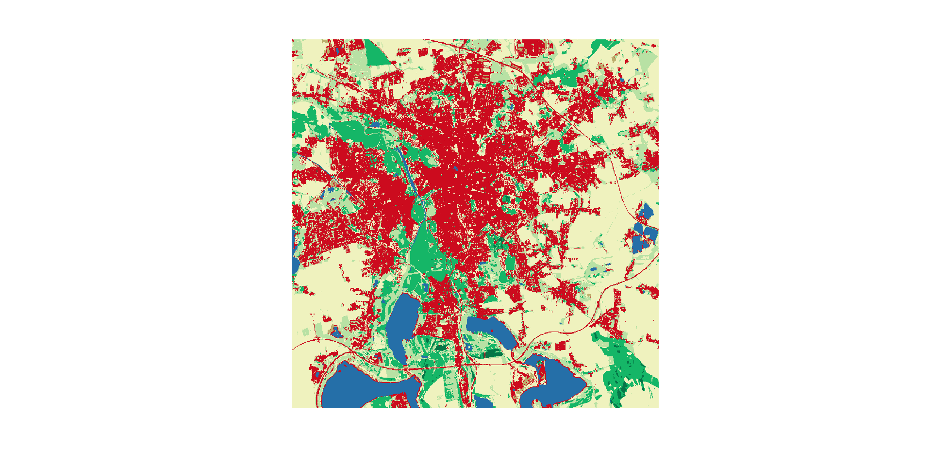

landcover <- rast("data/landcover-2015.tif") # this has 1 layer
ndvi <- rast("data/ndvi-2024.tif") # this has 10 layers, one per month
nlyr(ndvi)
[1] 10[1] 469 695 10Rasters
2025-06-26
rast(<filename>) to load a raster.rast() can also load them.landcover <- rast("data/landcover-2015.tif") # this has 1 layer
ndvi <- rast("data/ndvi-2024.tif") # this has 10 layers, one per month
nlyr(ndvi)[1] 10[1] 469 695 10Common raster file extensions are: .tif, .gif, .grib, .hd5, .nc (netCDF), and .png.
class       : SpatRaster
dimensions  : 469, 695, 10  (nrow, ncol, nlyr)
resolution  : 0.0004491576, 0.0004491576  (x, y)
extent      : 12.2338, 12.54596, 51.209, 51.41966  (xmin, xmax, ymin, ymax)
coord. ref. : lon/lat WGS 84 (EPSG:4326)
source      : ndvi-2024.tif
names       :    january,      march,      april,        may,       june,       july, ...
min values  : -0.8566782, -0.6070393, -1.0000000, -0.4106196, -1.0000000, -0.7984271, ...
max values : 0.8910936, 0.8981348, 0.9751282, 0.9380596, 0.9398647, 0.9476519, ... dimensions: size of the raster.resolution: horizontal resolution.extent: area covered by the raster.coord. ref.: coordinate reference system (CRS).names: names of the layers.Caution
Rasters without the same dimension, resolution, extent, or CRS cannot be combined.
Error: [rast] extents do not match
terra has functions to get the metadata in a programmatic way:
dim() for dimensions.res() for resolution.ext() for spatial extent.crs() for the CRS.names() for names.[1] "PROJCRS[\"ETRS89-extended / LAEA Europe\",\n BASEGEOGCRS[\"ETRS89\",\n ENSEMBLE[\"European Terrestrial Reference System 1989 ensemble\",\n MEMBER[\"European Terrestrial Reference Frame 1989\"],\n MEMBER[\"European Terrestrial Reference Frame 1990\"],\n MEMBER[\"European Terrestrial Reference Frame 1991\"],\n MEMBER[\"European Terrestrial Reference Frame 1992\"],\n MEMBER[\"European Terrestrial Reference Frame 1993\"],\n MEMBER[\"European Terrestrial Reference Frame 1994\"],\n MEMBER[\"European Terrestrial Reference Frame 1996\"],\n MEMBER[\"European Terrestrial Reference Frame 1997\"],\n MEMBER[\"European Terrestrial Reference Frame 2000\"],\n MEMBER[\"European Terrestrial Reference Frame 2005\"],\n MEMBER[\"European Terrestrial Reference Frame 2014\"],\n ELLIPSOID[\"GRS 1980\",6378137,298.257222101,\n LENGTHUNIT[\"metre\",1]],\n ENSEMBLEACCURACY[0.1]],\n PRIMEM[\"Greenwich\",0,\n ANGLEUNIT[\"degree\",0.0174532925199433]],\n ID[\"EPSG\",4258]],\n CONVERSION[\"Europe Equal Area 2001\",\n METHOD[\"Lambert Azimuthal Equal Area\",\n ID[\"EPSG\",9820]],\n PARAMETER[\"Latitude of natural origin\",52,\n ANGLEUNIT[\"degree\",0.0174532925199433],\n ID[\"EPSG\",8801]],\n PARAMETER[\"Longitude of natural origin\",10,\n ANGLEUNIT[\"degree\",0.0174532925199433],\n ID[\"EPSG\",8802]],\n PARAMETER[\"False easting\",4321000,\n LENGTHUNIT[\"metre\",1],\n ID[\"EPSG\",8806]],\n PARAMETER[\"False northing\",3210000,\n LENGTHUNIT[\"metre\",1],\n ID[\"EPSG\",8807]]],\n CS[Cartesian,2],\n AXIS[\"northing (Y)\",north,\n ORDER[1],\n LENGTHUNIT[\"metre\",1]],\n AXIS[\"easting (X)\",east,\n ORDER[2],\n LENGTHUNIT[\"metre\",1]],\n USAGE[\n SCOPE[\"Statistical analysis.\"],\n AREA[\"Europe - European Union (EU) countries and candidates. Europe - onshore and offshore: Albania; Andorra; Austria; Belgium; Bosnia and Herzegovina; Bulgaria; Croatia; Cyprus; Czechia; Denmark; Estonia; Faroe Islands; Finland; France; Germany; Gibraltar; Greece; Hungary; Iceland; Ireland; Italy; Kosovo; Latvia; Liechtenstein; Lithuania; Luxembourg; Malta; Monaco; Montenegro; Netherlands; North Macedonia; Norway including Svalbard and Jan Mayen; Poland; Portugal including Madeira and Azores; Romania; San Marino; Serbia; Slovakia; Slovenia; Spain including Canary Islands; Sweden; Switzerland; Turkey; United Kingdom (UK) including Channel Islands and Isle of Man; Vatican City State.\"],\n BBOX[24.6,-35.58,84.73,44.83]],\n ID[\"EPSG\",3035]]"[1] "+proj=laea +lat_0=52 +lon_0=10 +x_0=4321000 +y_0=3210000 +ellps=GRS80 +units=m +no_defs" name authority code
1 ETRS89-extended / LAEA Europe EPSG 3035
area
1 Europe - European Union (EU) countries and candidates. Europe - onshore and offshore: Albania; Andorra; Austria; Belgium; Bosnia and Herzegovina; Bulgaria; Croatia; Cyprus; Czechia; Denmark; Estonia; Faroe Islands; Finland; France; Germany; Gibraltar; Greece; Hungary; Iceland; Ireland; Italy; Kosovo; Latvia; Liechtenstein; Lithuania; Luxembourg; Malta; Monaco; Montenegro; Netherlands; North Macedonia; Norway including Svalbard and Jan Mayen; Poland; Portugal including Madeira and Azores; Romania; San Marino; Serbia; Slovakia; Slovenia; Spain including Canary Islands; Sweden; Switzerland; Turkey; United Kingdom (UK) including Channel Islands and Isle of Man; Vatican City State
extent
1 -35.58, 44.83, 84.73, 24.60This is done as if the layers were in a list.
<raster>[[i]] select the i-th layer.<raster>[[c(3, 6, 12)]] select the third, sixth, and 12th layers.class : SpatRaster
dimensions : 469, 695, 2 (nrow, ncol, nlyr)
resolution : 0.0004491576, 0.0004491576 (x, y)
extent : 12.2338, 12.54596, 51.209, 51.41966 (xmin, xmax, ymin, ymax)
coord. ref. : lon/lat WGS 84 (EPSG:4326)
source : ndvi-2024.tif
names : april, july
min values : -1.0000000, -0.7984271
max values : 0.9751282, 0.9476519 class : SpatRaster
dimensions : 469, 695, 1 (nrow, ncol, nlyr)
resolution : 0.0004491576, 0.0004491576 (x, y)
extent : 12.2338, 12.54596, 51.209, 51.41966 (xmin, xmax, ymin, ymax)
coord. ref. : lon/lat WGS 84 (EPSG:4326)
source : ndvi-2024.tif
name : march
min value : -0.6070393
max value : 0.8981348 This is done as if the layers were matrices.
<raster>[i, j] select the value in row i and column j january march april may june july august september
1 0.7144094 0.8246858 0.5798226 0.8630141 0.236645 0.517687 0.7169055 0.1734121
october december
1 0.7473408 0.8695881Note
We will see a better way of doing this later
This is done using the default R operator c().
c(<raster-a>, <raster-b>) combines the layers of the two rasters.class : SpatRaster
dimensions : 469, 695, 2 (nrow, ncol, nlyr)
resolution : 0.0004491576, 0.0004491576 (x, y)
extent : 12.2338, 12.54596, 51.209, 51.41966 (xmin, xmax, ymin, ymax)
coord. ref. : lon/lat WGS 84 (EPSG:4326)
sources : ndvi-2024.tif
ndvi-2024.tif
names : january, april
min values : -0.8566782, -1.0000000
max values : 0.8910936, 0.9751282 rast(<filename>).writeRaster(<raster>, <filename>)Note
By default, overwrite = FALSE and writeRaster() will stop if the file already exists.
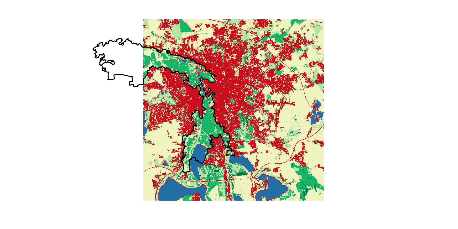
I want to plot the geometry of the forest on top of landcover
Where is the forest?
Tip
When something does not work, check the metadata.
[1] "+proj=laea +lat_0=52 +lon_0=10 +x_0=4321000 +y_0=3210000 +ellps=GRS80 +units=m +no_defs"[1] "+proj=longlat +datum=WGS84 +no_defs"The CRS does not match.
What is this project()?
Gui will explain after the break.