Introduction to GIS

Raster Operations

2025-06-27

Operations

Summary statistics: calculate some metric.
Aggregation and disaggregation: combine/split multiple cells.
Resampling: resample cell values to another grid.
Extraction and masking: get values from geometries.

Summary statistics

Local summary: across pixels of different layers at the same location.
Global summary: across all pixels of one layer.
Zonal summary: across all pixels within one zone.

Local summary

Calculate a summary for pixels with the same location across layers.

ndvi <- rast("data/ndvi-2024.tif")
plot(
  ndvi[[1:3]],
  nr = 1,
  col = hcl.colors(100, "Fall", rev = TRUE),
  frame = FALSE, axes = FALSE
)

Local summary

Calculate a summary for pixels with the same location across layers.

In terra you can use some basic functions, such as mean(), sum(), etc.

avg_ndvi <- mean(ndvi, na.rm = TRUE)
plot(avg_ndvi, col = hcl.colors(100, "Fall", rev = TRUE), frame = FALSE, axes = FALSE)

Local summary

Calculate a summary for pixels with the same location across layers.

In terra you can use some basic functions, such as mean(), sum(), etc.

For other function, you need to use app().

ndvi <- rast("data/ndvi-2024.tif")
greenest_month <- app(ndvi, "which.max", na.rm = TRUE) # layer ID with maximum NDVI
plot(
  greenest_month,
  type = "classes",
  col = hcl.colors(10, "Viridis"),
  frame = FALSE, axes = FALSE
)

Global summary

Global summaries are calculated across all pixels of a layer.

In terra you can use global(<raster>, <function>).

global(ndvi, "mean", na.rm = TRUE)

               mean
january   0.3887426
march     0.4403890
april     0.5492637
may       0.5802602
june      0.5067746
july      0.4962943
august    0.4762506
september 0.4215684
october   0.4762810
december  0.4690120

Zonal summary

Zonal statistics summarize the values of a raster using categories from another raster or geometry.

In terra, you can use zonal(<x>, <y>), where <x> is the raster with the values to summarize and <y> the raster/geometry specifying the zones.

landcover <- rast("data/landcover_4326-2015.tif")
avg_ndvi <- project(avg_ndvi, landcover)  # this will also resample avg_ndvi (see the section Resampling)
zonal(avg_ndvi, landcover, fun = "mean", na.rm = TRUE)

                   category       mean
1           Artificial Land  0.3972677
2                 Open Soil  0.1917675
3  High Seasonal Vegetation  0.7299292
4 High Perennial Vegetation  0.7495042
5   Low Seasonal Vegetation  0.5193868
6  Low Perennial Vegetation  0.6483166
7                     Water -0.2462283

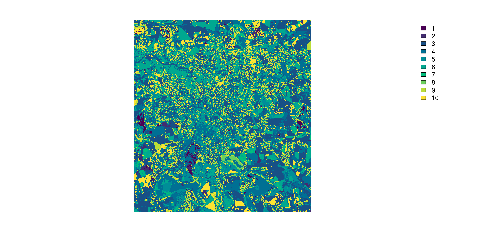
Zonal summary

Push it a bit further.

ndvi_landcover <- zonal(avg_ndvi, landcover, fun = "mean", na.rm = TRUE)
ndvi_landcover$sd <- zonal(avg_ndvi, landcover, fun = "sd", na.rm = TRUE)[, 2]
ndvi_landcover

                   category       mean         sd
1           Artificial Land  0.3972677 0.14956025
2                 Open Soil  0.1917675 0.18361272
3  High Seasonal Vegetation  0.7299292 0.04675755
4 High Perennial Vegetation  0.7495042 0.05914027
5   Low Seasonal Vegetation  0.5193868 0.09874814
6  Low Perennial Vegetation  0.6483166 0.09384940
7                     Water -0.2462283 0.27004502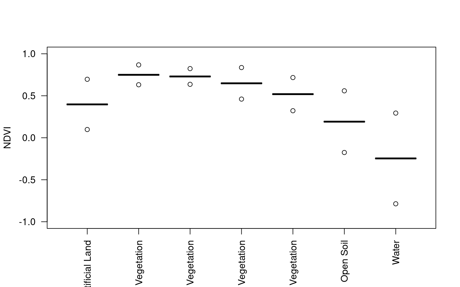

with(ndvi_landcover, plot(
  as.factor(category), mean,
  ylim = c(-1, 1), las = 2,
  xlab = "",
  ylab = "NDVI"
))
with(ndvi_landcover, points(as.factor(category), mean - 2 * sd))
with(ndvi_landcover, points(as.factor(category), mean + 2 * sd))

Aggregate & disaggregate

Aggregating creates a raster at coarser resolution.
Disaggregating creates a raster at finer resolution.

Aggregate

Use aggregate(<raster>, <fact>, <fun>) to aggregate rasters.

<fact> is the number of cells in each direction to be aggregated.
<fun> is the function used for aggregatation.

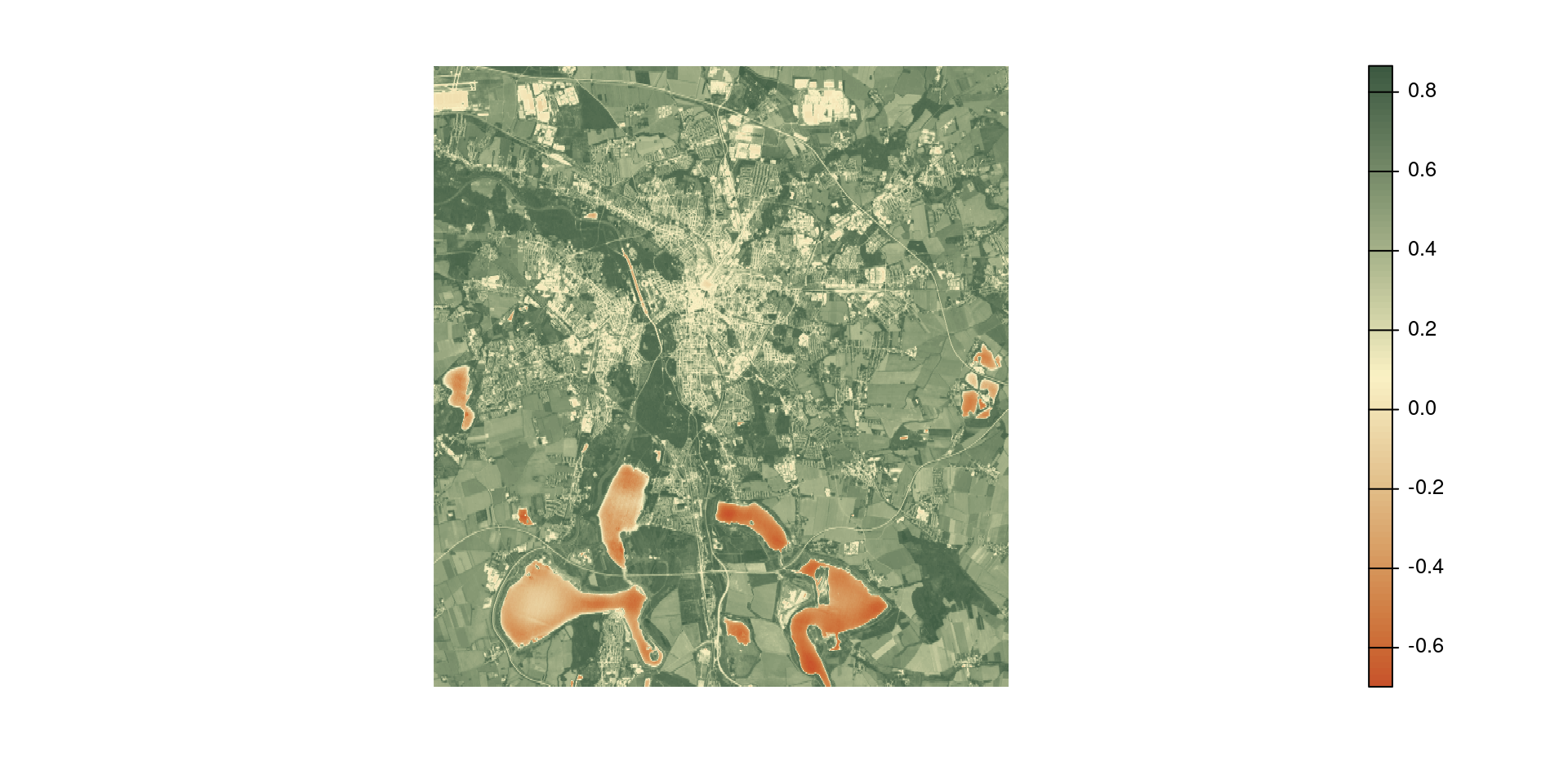
avg_ndvi_aggr <- aggregate(avg_ndvi, 25, "mean")
par(mfrow = c(1, 2))  # cannot stack rasters with different resolution
plot(avg_ndvi, col = hcl.colors(100, "Fall", rev = TRUE), frame = FALSE, axes = FALSE)
plot(avg_ndvi_aggr, col = hcl.colors(100, "Fall", rev = TRUE), frame = FALSE, axes = FALSE)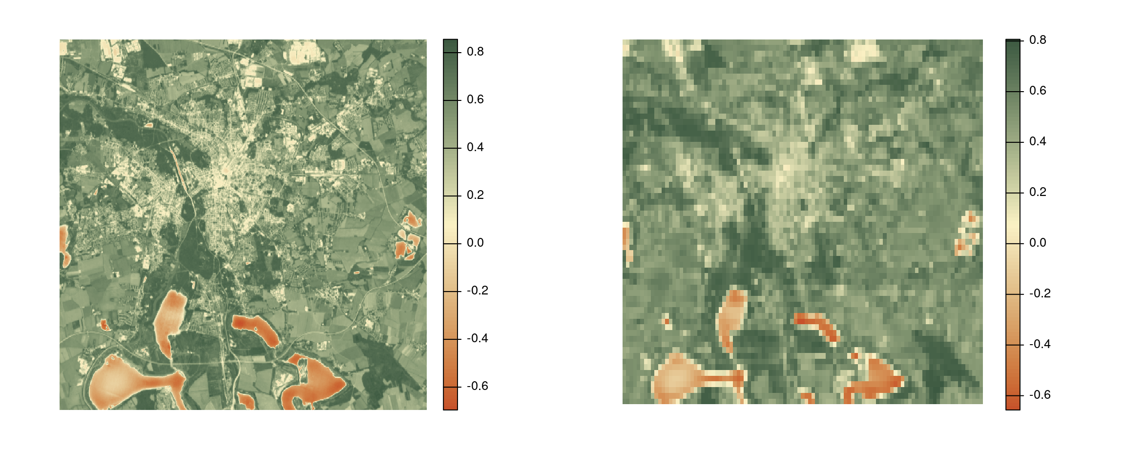

res(avg_ndvi_aggr) / res(avg_ndvi)

[1] 25 25

par(mfrow = c(1, 1))

Disaggregate

Use disagg(<raster>, <fact>, <method>) to aggregate rasters.

<fact> is the number of cells in each direction to be aggregated.
<method> is the method used for disaggregatation.

avg_ndvi_disaggr <- disagg(avg_ndvi_aggr, 25, "bilinear")
par(mfrow = c(1, 3))  # cannot stack rasters with different resolution
plot(avg_ndvi, col = hcl.colors(100, "Fall", rev = TRUE), frame = FALSE, axes = FALSE)
plot(avg_ndvi_aggr, col = hcl.colors(100, "Fall", rev = TRUE), frame = FALSE, axes = FALSE)
plot(avg_ndvi_disaggr, col = hcl.colors(100, "Fall", rev = TRUE), frame = FALSE, axes = FALSE)

res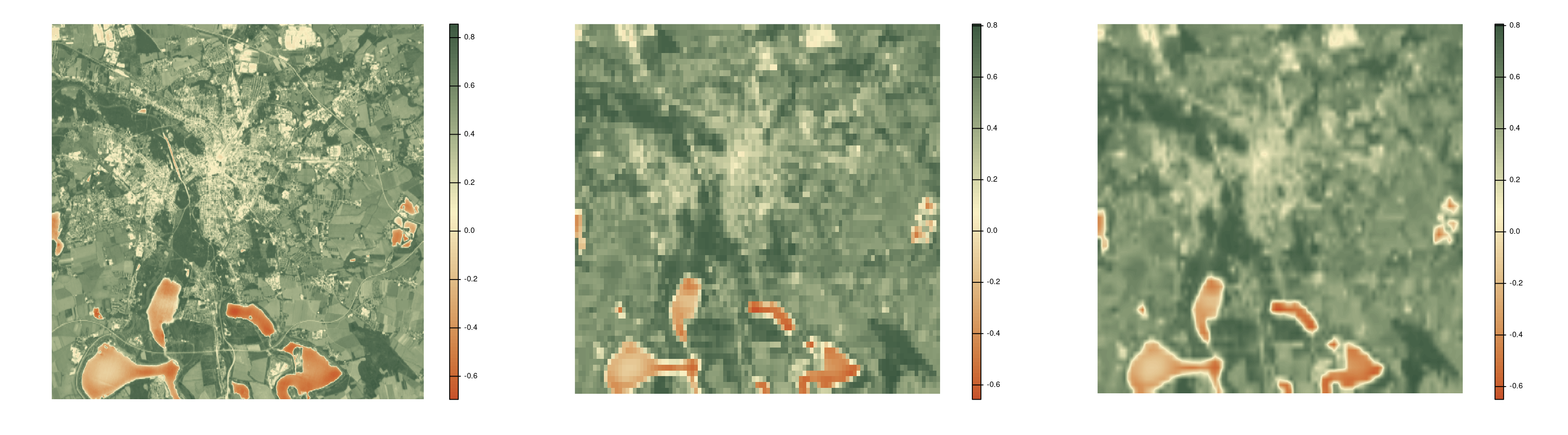(avg_ndvi_disaggr) / res(avg_ndvi)

[1] 1 1

Disaggregating aggregating rasters

Caution

disaggr() and aggregate() are not inverse functions.

Aggregating and disaggregating a raster does not give, in general, the same raster back. Some of the original information is lost during aggregation.

r <- rast(matrix(rnorm(16^2), 16, 16), crs = "EPSG:4326")
plot(
  c(r, r |> aggregate(4, "mean") |> disagg(4, "bilinear")),
  col = hcl.colors(100, "Viridis"),
  axes = FALSE, frame = FALSE
)

Resampling

Resampling transform one raster into a raster that align with another raster.
Useful when two rasters do not align, i.e. they have different origin or resolution.

Resampling

resample(<x>, <y>, <method>) resamples raster <x> to raster <y>.

<method> is used to specify the algorithm used for resampling:

- `near`, for nearest neighbor.
- `bilinear`, for bilinear interpolation.
- `cubic`, for cubic interpolation.
- `cubicspline`, for cubic-spline interpolation.
- `lanczos`, for Lanczos resampling.

ndvi <- rast("data/ndvi-2024.tif")
landcover <- rast("data/landcover_4326-2015.tif")

ndvi <- resample(ndvi, landcover, method = "bilinear")
avg_ndvi <- mean(ndvi)
zonal(avg_ndvi, landcover, fun = "mean", na.rm = TRUE)

                   category       mean
1           Artificial Land  0.3972643
2                 Open Soil  0.1917675
3  High Seasonal Vegetation  0.7299290
4 High Perennial Vegetation  0.7495042
5   Low Seasonal Vegetation  0.5193560
6  Low Perennial Vegetation  0.6483423
7                     Water -0.2462283

Resampling

project(<x>, <y>) performs an implicit resampling when <y> is a raster and <x> and <y> do not align.

Note

project(<x>, crs(<y>)) projects only the CRS.

project(<x>, <y>) actually resamples <x> to <y>.

In many cases resample(<x>, <y>, <method>) can be avoided by using project(<x>, <y>, <method>).

Explicit is better than implicit.

Operation on rasters and geometries

Extract values from a raster.
Crop the extent of a raster.
Mask a raster.

Extract values

extract(<x>, <y>) extract the values from raster <x> for the geometries of <y>.

idiv <- vect("data/idiv.shp")
ndvi <- rast("data/ndvi-2024.tif") |> mean()
extract(ndvi, idiv, cells = TRUE, xy = TRUE)

  ID      mean   cell        x        y
1  1 0.2571441 156737 12.39617 51.31837
2  1 0.3292601 157432 12.39617 51.31792

The options cell = TRUE and xy = TRUE return also the cell ID and the coordinates x and y.

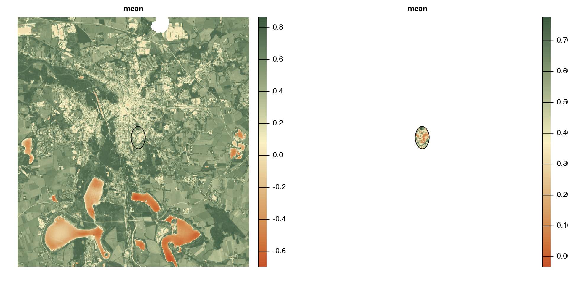
Crop a raster

crop(<x>, <y>) crop the extent of raster <x> to the extent of <y>.

idiv_buffer <- buffer(idiv, 1e3)

ndvi_cropped <- crop(ndvi, idiv_buffer)
plot(ndvi_cropped, col = hcl.colors(100, "Fall", rev = TRUE), axes = FALSE, frame = FALSE)
lines(idiv_buffer)

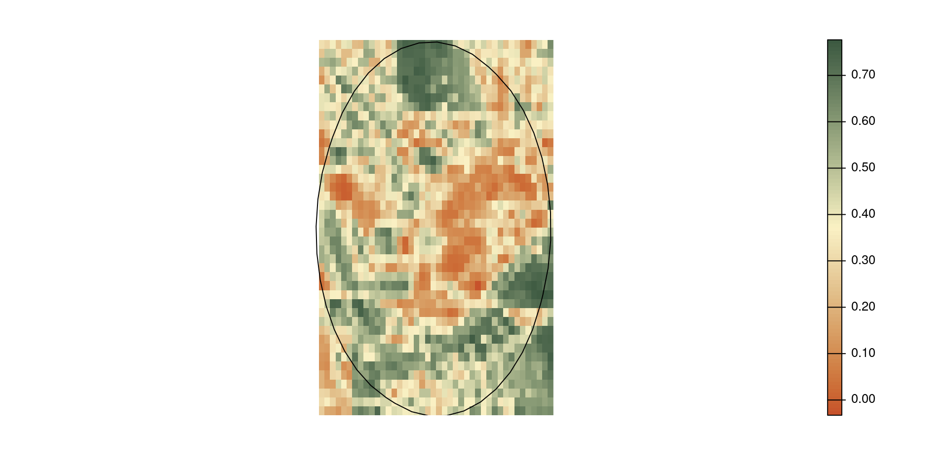
Mask a raster

mask(<x>, <y>) mask the cells of raster <x> to <y>.

mask() does not crop the extent.

If <y> is a geometry, cells outside the geometries are set to NA.

ndvi_masked <- mask(ndvi, idiv_buffer)
plot(
  c(ndvi, ndvi_masked),
  fun = function() lines(idiv_buffer),  # draw the buffer on each panel
  col = hcl.colors(100, "Fall", rev = TRUE), axes = FALSE, frame = FALSE
)

Exercise

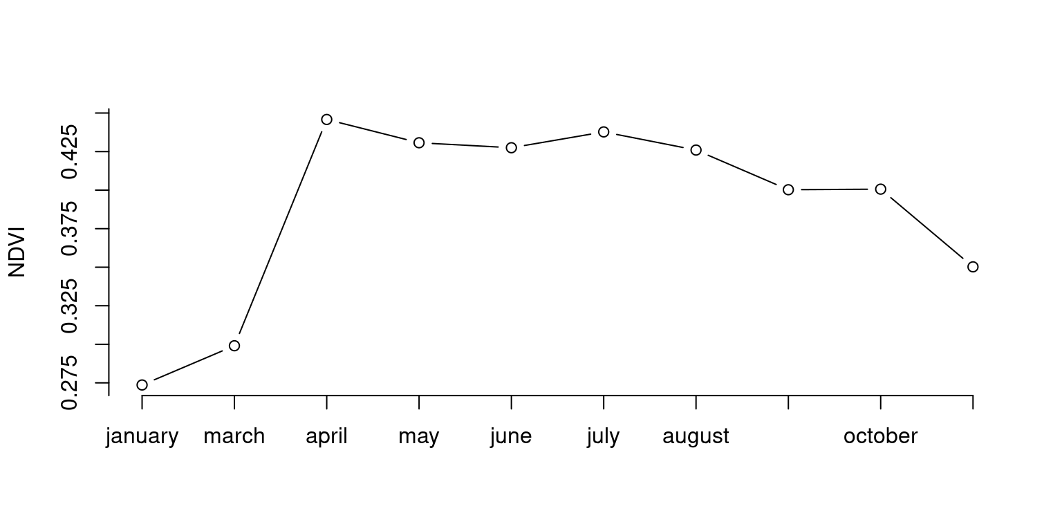
Plot the trend of NDVI during the year for the area within 1 km distance from the iDiv building .

Show the code

roi <- vect("data/idiv.shp") |> buffer(1e3)
ndvi <- rast("data/ndvi-2024.tif")
trend <- ndvi |> 
  mask(roi) |> 
  global("mean", na.rm = TRUE)
trend$month <- rownames(trend)
plot(
  seq_along(trend$month),
  trend$mean,
  xlab = "",
  ylab = "NDVI",
  type = "b",
  axes = FALSE
)
axis(1, seq_along(trend$month), trend$month)
axis(2, seq(-1, 1, by = .025), seq(-1, 1, by = .025))