 [1] "gbifID"                           "datasetKey"
 [3] "occurrenceID"                     "kingdom"
 [5] "phylum"                           "class"
 [7] "order"                            "family"
 [9] "genus"                            "species"
[11] "infraspecificEpithet"             "taxonRank"
[13] "scientificName"                   "verbatimScientificName"
[15] "verbatimScientificNameAuthorship" "countryCode"
[17] "locality"                         "stateProvince"
[19] "occurrenceStatus"                 "individualCount"
[21] "publishingOrgKey"                 "decimalLatitude"
[23] "decimalLongitude"                 "coordinateUncertaintyInMeters"
[25] "coordinatePrecision"              "elevation"
[27] "elevationAccuracy"                "depth"
[29] "depthAccuracy"                    "eventDate"
[31] "day"                              "month"
[33] "year"                             "taxonKey"
[35] "speciesKey"                       "basisOfRecord"
[37] "institutionCode"                  "collectionCode"
[39] "catalogNumber"                    "recordNumber"
[41] "identifiedBy"                     "dateIdentified"
[43] "license"                          "rightsHolder"
[45] "recordedBy"                       "typeStatus"
[47] "establishmentMeans"               "lastInterpreted"
[49] "mediaType" "issue" Introduction to GIS
Example: species distribution model
2025-06-27
Before we start
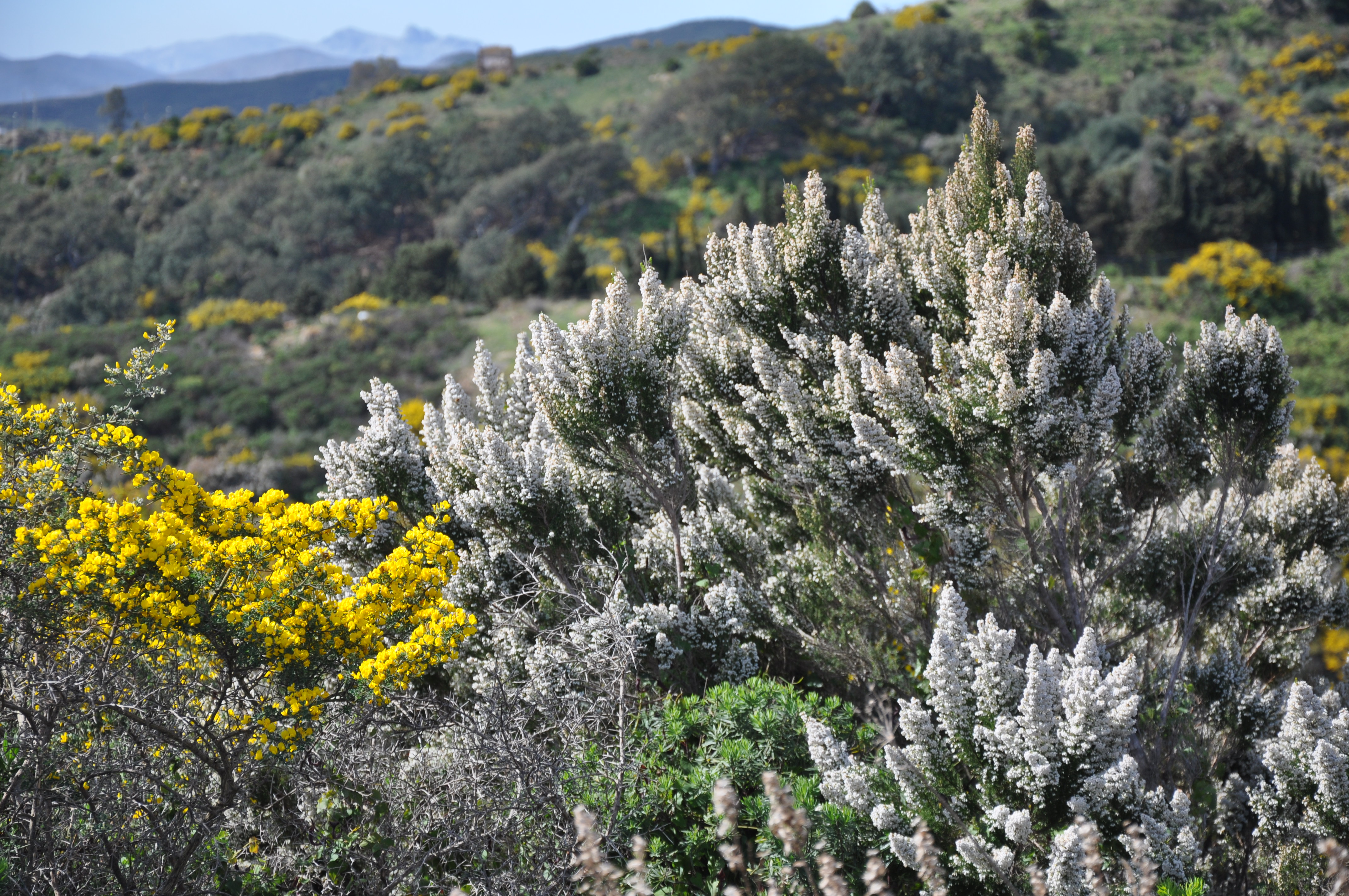
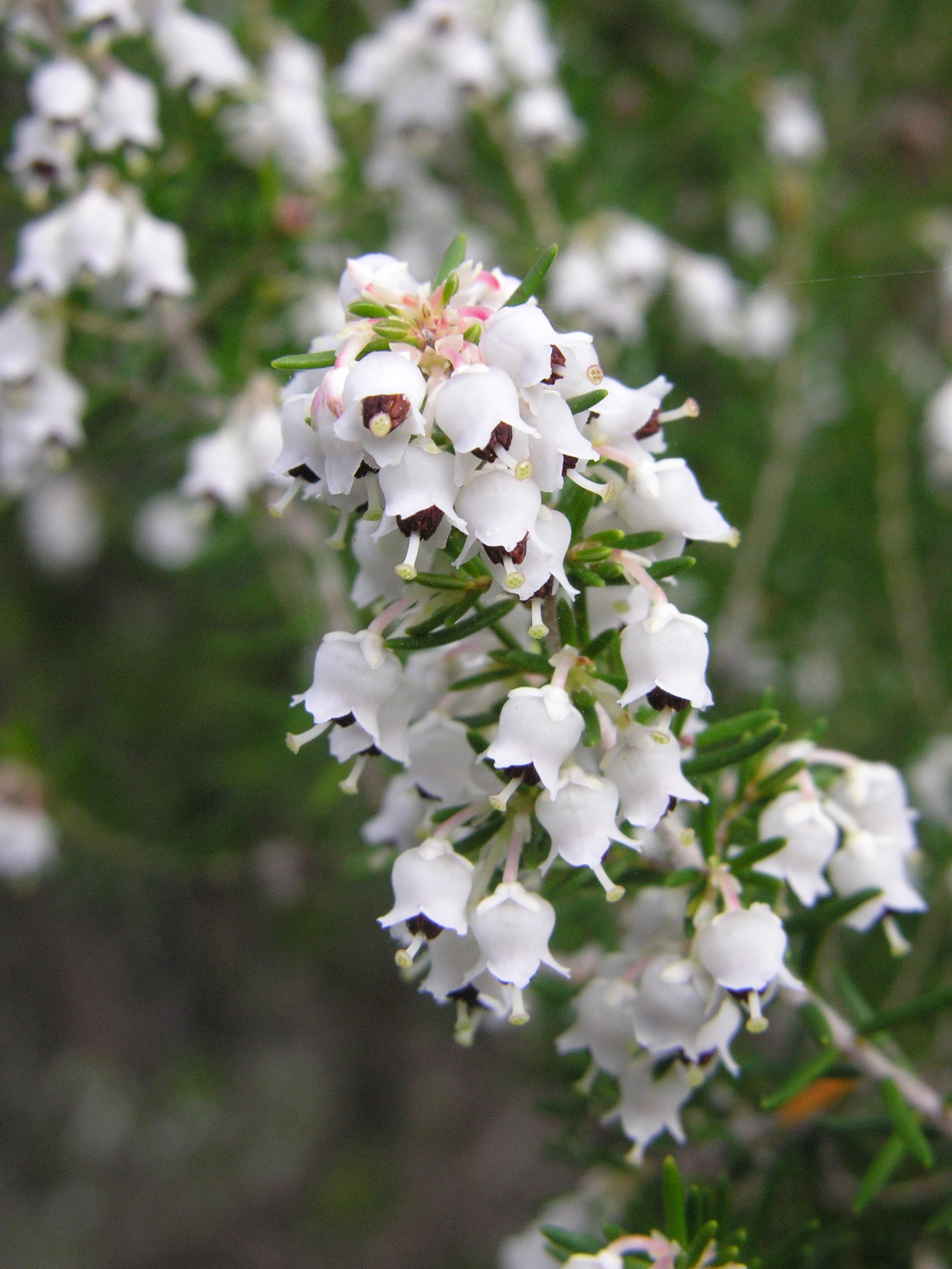
- Choose one species you are interested in: Erica arborea.
Before we start
- Choose one species you are interested in: Erica arborea.
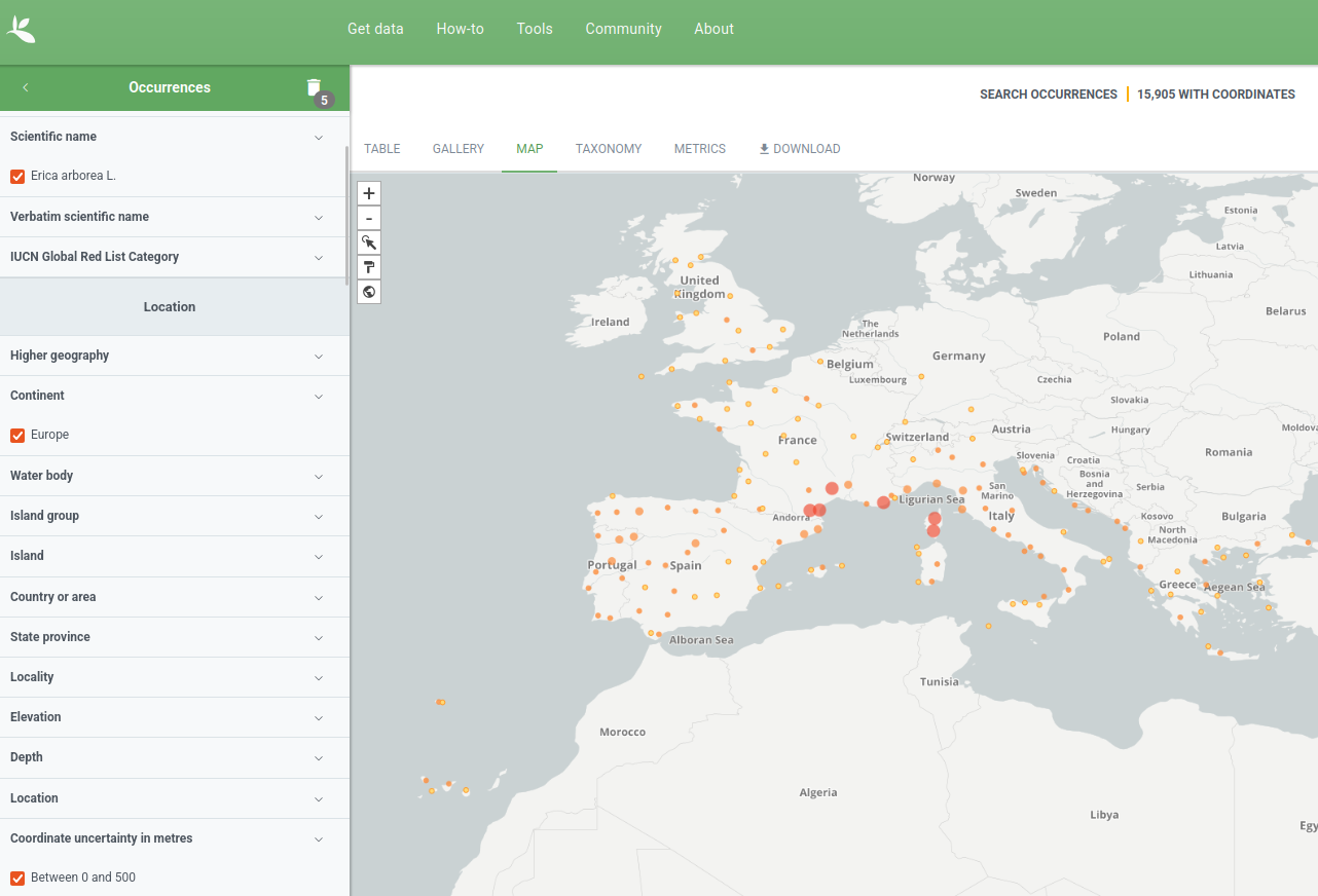
- Go to gbif.org and download the occurrence.
Before we start
- Choose one species you are interested in: Erica arborea.
- Go to gbif.org and download the occurrence.
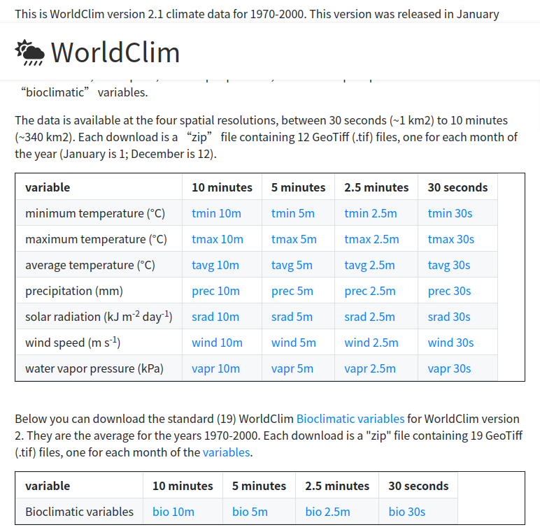
- Go to worldclim.org and download the bioclimatic variables at 5 arc-minute resolution (https://geodata.ucdavis.edu/climate/worldclim/2_1/base/wc2.1_5m_bio.zip).
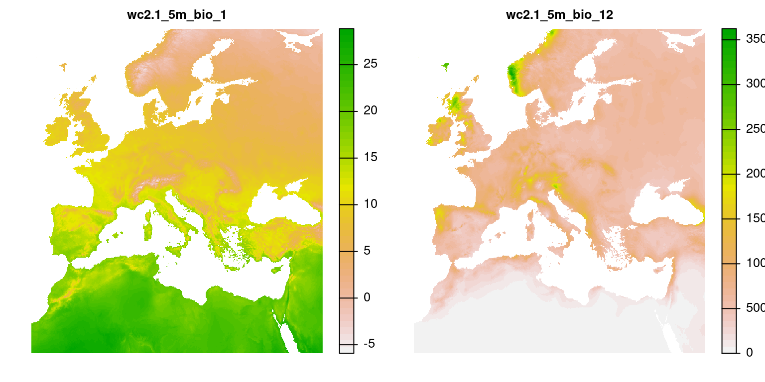
Load climate data
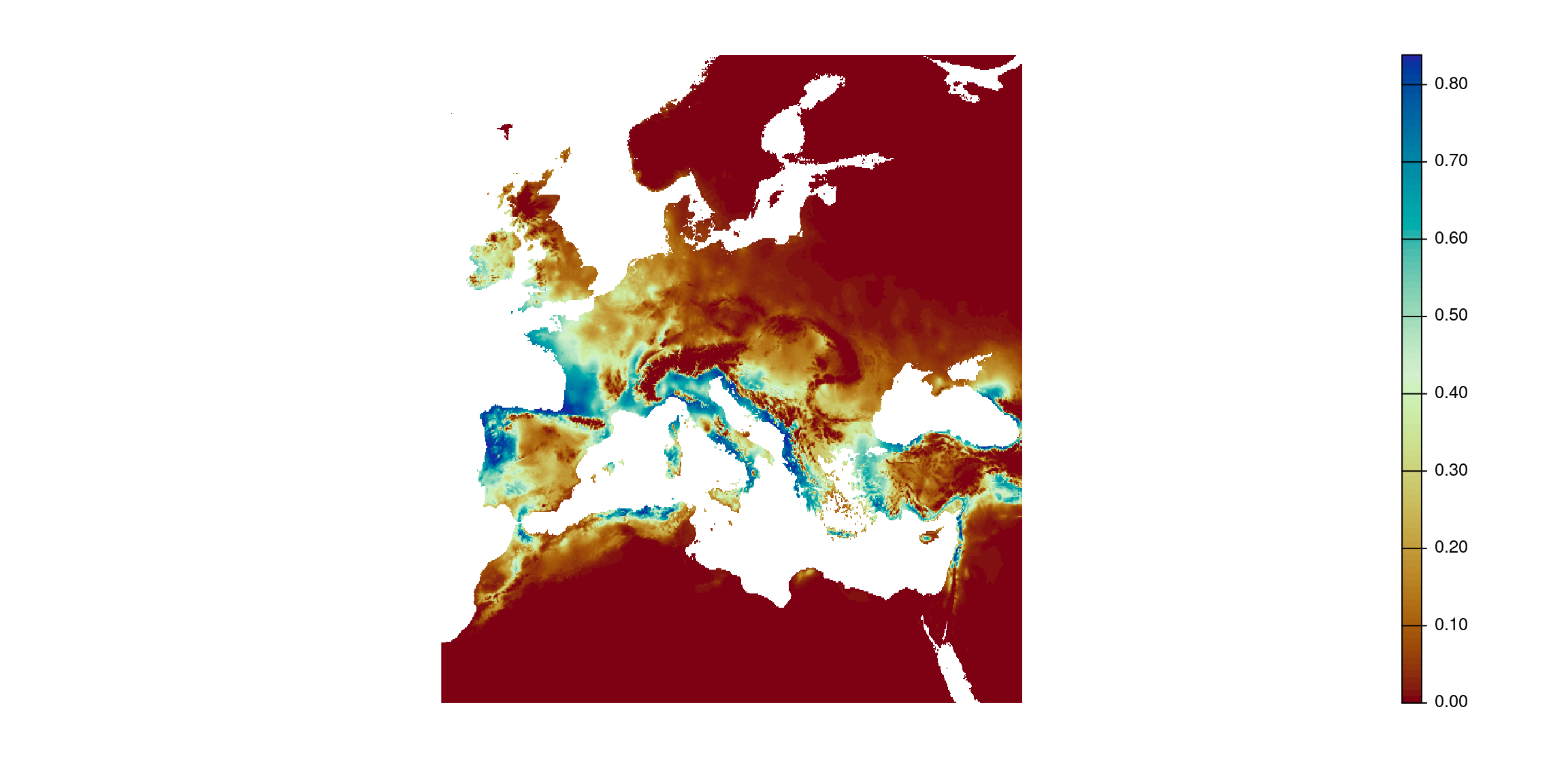
Potential distribution