Emilio Berti
![]()
![]()
![]()
Getting started
Background
Following food web terminology, I talk here about resources and consumers. In the case of plant-pollinator networks, this is analogous as replacing resources with plants and consumers with pollinators. In this case, however, some filtering steps may be unnecessary or unwanted. More about this in a separate section. I also talk about metawebs, which are the regional food web networks that emerge considering all interactions that occur in local communities within the region of interest.
The main scope of assembly is to simulate top-down assembly processes. Top-down assembly means that all species are introduced into a local community at once. The opposite, i.e. communities are built by sequential introductions of one species, is called bottom-up assembly. Bottom-up assembly is problematic for community composed of many species, as the number of unique assembly sequences is S!, where S is the number of species in the metaweb. If priority effects (historical contigencies) are important, Song, Fukami, and Saavedra (2021) found that this number is (much) higher, roughly:
Thus, for a conservative scenario where priority effects are not
important in a 100 species community, there are
unique sequences, making computations (and replications) virtually
impossible. With priority effects, “already with 6 species, the
diversity is significantly greater than the total number of atoms in the
entire universe” (Song, Fukami, and Saavedra (2021)).
Strikingly, Serván and Allesina (2021) showed that bottom-up and top-down assembly are equivalent under some specific conditions. Far from assuming this is the case in assembly, for which more research is needed, I simply want to highlight that assembly only implements top-down assembly and that none of the procedures in assembly can be considered steps in an ecological sequence. Whenever I talk about steps, moves, and sequences in assembly, I always refer to procedures steps, procedures moves, and procedures sequences. Always keep that in mind and don’t be fooled by the terminology; there is no bottom-up assembly in assembly.
At this point, if you’re like me, you will ask why not bottom-up
assembly? The simple answer is: because it is computational unfeasible
for large communities. To make it feasible, it is tempting to restrict
the possible sequences to a (very) narrow space, only to 1,000,000
sequences
(
of the total fraction of possible sequences for 100 species; much much
smaller than considering only a grain of sand for simulating the whole
Earth). As this seems quite dangerous, potentially leading to biased
conclusions, I completed neglected bottom-up assembly processes.
General workflow of assembly
In general, assembly implements this pipeline:
- Draw random species from a metaweb.
- Impose resource filtering, i.e. each basal species must be consumed and each consumer must feed on a resource.
- Impose limiting similarity filtering, i.e. consumers are replaced by others, depending on a probability distribution proportional to their similarity of interactions.
These steps are not necessarily sequential, i.e. limiting similarity can be imposed independently from the resource filtering, but this is programmatically harder. Because ecological communities are likely filtered by resource availability before interaction competition, I wrote assembly in a way that is straightforward to pass the output of the resource filtering procedure to the limiting similarity one. It is, however, possible to omit/invert procedures by performing extra-checks on input/output data and implementing few pre-procedure steps. I will show how to implement some of them at the end.
Draw random species from a metaweb
Loading assembly and set a random seed
library(assembly)
library(igraph)
#>
#> Attaching package: 'igraph'
#> The following objects are masked from 'package:stats':
#>
#>     decompose, spectrum
#> The following object is masked from 'package:base':
#>
#>     union

set.seed(123)
Load the dataset adirondack that comes with assembly:
data(adirondack)
adirondack is the Adirondack Lakes metaweb as obtained from the GATEWAy database.
draw_random_species(n, sp.names) draws random species from a metaweb
and requires as input the number of species to draw (n) and the
species names (sp.names). If the metaweb does not have species names,
you can assign random ones with name_metaweb(metaweb):
colnames(name_metaweb(matrix(as.numeric(runif(100) > .5), 10, 10)))
#>  [1] "ytvynywchp" "lyncngcwvz" "ouehsjrjlb" "jvltnqnvch" "nsoxqwkgow"
#>  [6] "zfngjefpxu" "wkdlnsygvz" "igbpmsxtog" "dahtypxvkp" "thcdtlvqjt"
If names are already present, this will throw an error:
tryCatch(name_metaweb(adirondack),
         error = function(e) print(e))
#> <simpleError in name_metaweb(adirondack): Names are already present>
When the metaweb has names, define the number of species for the local community:
S <- 50 #species richness
And draw a random community, use the function draw_random_species():
sp <- draw_random_species(S, colnames(adirondack))
show_graph(sp, adirondack)
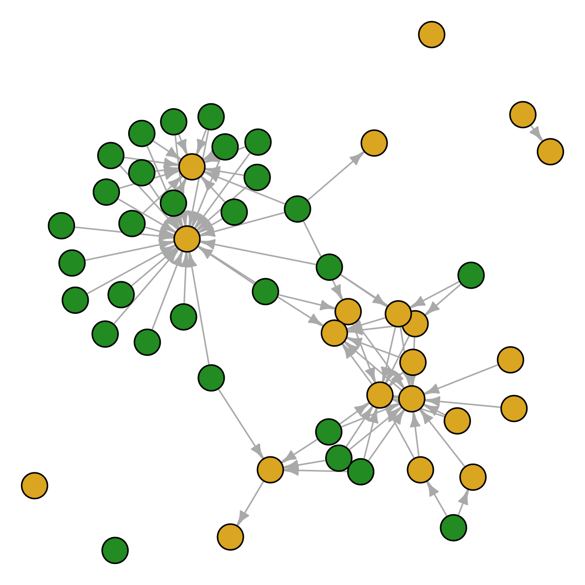
Hidden functions
There are several hidden functions in assembly. The reason there are
hidden functions is because there is no need to call them directly.
Hidden functions can be accessed by prefixing the assembly::: (three
colon, not two). All hidden functions start with a dot .,
e.g. assembly:::.basals().
In general, you should not be bothered by hidden functions and should not call them directly, unless you have a good understanding of how they operate. Nevertheless, I summarize them for clarity.
assembly:::.basals() get all basal species in the metaweb, and is
equivalent to subset the names of the metaweb where
colSums(metaweb) == 0:
identical(
  sort(intersect(assembly:::.basals(adirondack), sp)),
  sort(intersect(colnames(adirondack)[colSums(adirondack) == 0], sp))
)
#> [1] TRUE
assembly:::.consumers() and assembly:::.top() return the consumers
and top consumers of the metaweb, respectively.
assembly:::.find_isolated() returns the species that are isolated in
the local community:
assembly:::.find_isolated(sp, adirondack)
#> [1] "Halotheca sp."             "Conochiloides hippocrepis"
#> [3] "Keratella serrulata"       "Ceriodaphnia quadrangula"
#> [5] "Polyarthra euryptera"      "Lepadella triptera"
#> [7] "Prosopium cylindraceum"    "Catostomus catostomus"
assembly:::.find_replacements() find suitable replacement for the
isolated species:
assembly:::.find_replacements(sp,
                              assembly:::.find_isolated(sp, adirondack),
                              adirondack,
                              keep.n.basal = TRUE)
#> [1] "Ploesoma hudsoni"            "fish fry"
#> [3] "Salmo rutta"                 "Conochiloides unicornis"
#> [5] "Keratella crassa"            "Coregonus artedii"
#> [7] "Salvelinus fontinalis small" "Chroococcus sp."
If keep.n.basal is TRUE (default = FALSE), then the original number of basal species will not change.
assembly:::.move() performs a move in the limiting similarity
procedure (more about this later):
tryCatch(assembly:::.move(sp, adirondack, t = 1),
         error = function(e) print(e))
#>  [1] "Cosmarium sp."               "Alona costata"
#>  [3] "Anabaena flos-aquae"         "Fragilaria sp."
#>  [5] "Holopedium gibberum"         "Quadrigula closterioides"
#>  [7] "Crucigenia quadrata"         "Chlamydomonas sp."
#>  [9] "Chrysosphaerella longispina" "Euchlanis sp."
#> [11] "Arthrodesmus octocornis"     "Euglena acus"
#> [13] "Halotheca sp."               "Cyclops scutifer"
#> [15] "Polyarthra major"            "Staurastrum megacanthum"
#> [17] "Conochiloides hippocrepis"   "Scenedesmus sp."
#> [19] "Crucigenia crucifera"        "Bosmina longirostris"
#> [21] "Ascomorpha ecaudis"          "Sida crystallina"
#> [23] "Pediastrum tetras"           "Rhinichthys atratulus"
#> [25] "Schroederia setigera"        "Dinobryon sp."
#> [27] "Cocconeia sp."               "Euastrum sp."
#> [29] "Fragilaria crotonensis"      "Sphaerocystis schroeteri"
#> [31] "Peridinium wisconsinense"    "Keratella serrulata"
#> [33] "Ceriodaphnia quadrangula"    "Oncorhynchus mykiss"
#> [35] "Daphnia galeata"             "Polyarthra euryptera"
#> [37] "Micropterus salmoides"       "Peridinium limbatum"
#> [39] "Microsystis sp."             "Pimephales promelas"
#> [41] "Lepadella triptera"          "Tropocyclops prasinus"
#> [43] "Peridinium inconspicuum"     "Carteria sp."
#> [45] "Prosopium cylindraceum"      "Tabellaria flocculosa"
#> [47] "Aphanothece sp."             "Diatoma sp."
#> [49] "Catostomus catostomus"       "Micrasterias sp."
This call to assembly:::.move() fails because isolated species are
detected in the input. This is a desired property of the function,
i.e. it fails when there is an unexpected behavior. All hidden functions
have some kind of behavior-check, which is a safety net to assure the
code is doing what you asked for.
Finally, assembly:::.components() returns the number of connected
components in the graph of the local community:
assembly:::.components(sp, adirondack)
#> [1] 5
Usually, a proper food web has only one component, i.e. all species are connected by a path. Having more than one component means that the food web is actually made of several disconnected communities. In the case above, it also means that at least one of this disconnected communities is composed of only one isolated species.
Resource filtering
To impose the resource filtering, call the function
resource_filtering(). This takes as input the species names
(sp.names), the metaweb (metaweb), and an optional argument
keep.n.basal to specify weather the original number of basal species
should be kept constant (default = FALSE). NOTE this may not be
implemented correctly
Behind the curtain, resource_filtering() calls the hidden functions as
a way to compress code and make it consistent. That’s why you shouldn’t
bother too much about hidden functions: they’re there because they’re
useful in the development of the package, rather than for your usage. If
they’re useful for you and you understand how they work, use them.
sp_resource <- resource_filtering(sp, adirondack, keep.n.basal = TRUE)
show_graph(sp_resource, adirondack)

Now the local community is fully connected, i.e. basal species always have a consumer and consumers always have an available resource. It’s possible to check this manually calling the hidden functions and working on the adjacency matrix of the local community:
bas <- intersect(sp_resource, assembly:::.basals(adirondack))
cons <- intersect(sp_resource, assembly:::.consumers(adirondack))
all(rowSums(adirondack[bas, cons]) > 0)
#> [1] TRUE
all(colSums(adirondack[union(bas, cons), cons]) > 0)
#> [1] TRUE
Usually you don’t need to perform these checks, as I implemented them
within resource_filtering(). I also implemented a check for
disconnected components, to make sure that the resulting community has
no isolated species and only one actual community.
Bonus: because of these checks, now it is safe to perform a move of the limiting similarity procedure:
assembly:::.move(sp_resource, adirondack, t = 1)
#>  [1] "Cosmarium sp."               "Alona costata"
#>  [3] "Anabaena flos-aquae"         "Fragilaria sp."
#>  [5] "Holopedium gibberum"         "Quadrigula closterioides"
#>  [7] "Crucigenia quadrata"         "Chlamydomonas sp."
#>  [9] "Chrysosphaerella longispina" "Euchlanis sp."
#> [11] "Arthrodesmus octocornis"     "Euglena acus"
#> [13] "Cyclops scutifer"            "Polyarthra major"
#> [15] "Staurastrum megacanthum"     "Scenedesmus sp."
#> [17] "Crucigenia crucifera"        "Bosmina longirostris"
#> [19] "Ascomorpha ecaudis"          "Sida crystallina"
#> [21] "Pediastrum tetras"           "Rhinichthys atratulus"
#> [23] "Schroederia setigera"        "Dinobryon sp."
#> [25] "Cocconeia sp."               "Euastrum sp."
#> [27] "Fragilaria crotonensis"      "Sphaerocystis schroeteri"
#> [29] "Peridinium wisconsinense"    "Oncorhynchus mykiss"
#> [31] "Daphnia galeata"             "Micropterus salmoides"
#> [33] "Peridinium limbatum"         "Microsystis sp."
#> [35] "Pimephales promelas"         "Tropocyclops prasinus"
#> [37] "Peridinium inconspicuum"     "Carteria sp."
#> [39] "Tabellaria flocculosa"       "Aphanothece sp."
#> [41] "Diatoma sp."                 "Micrasterias sp."
#> [43] "Salmo rutta"                 "Kelicottia bostoniensis"
#> [45] "fish fry"                    "Rhizosolenia eriensis"
#> [47] "Diaptomus minutus"           "Colletheca mutabilis"
#> [49] "Lepomis gibbosus"            "Keratella taurocephala"
Limiting similarity filtering
The limiting similarity filtering is a series of individuals moves. Each move is composed of three steps:
- A metric
(
) representing the similarity of interaction is calculated for each species in the community.
- One species is removed with probability proportional to their
- The species removed is replaced by another species selected at random from the metaweb.
Each move can then be accepted of discarded based on a probabilistic acceptance criterion, the Metropolis-Hasting algorithm (see below for details). If the move is accepted, the new community will differ from the starting one only in the removed/replaced species. If the move is discarded, the new community is identical to the starting one. Each move takes as input the community of the previous move (or the initial community for the first move) and returns as output the new community (or the original one).
The limiting similarity procedure is simply a series of moves (accepted or not). The starting community for the limiting similarity procedure is usually a community that has undergone already a resource filtering, imposing thus that trophic competition comes after resource availability. However, it is possible to skip the resource filtering step; the only requirement of the starting community for the limiting similarity filtering is that it does not have isolated species and has only one connected components.
To impose the limiting similariy filtering, call the function
similarity_filtering(). This function requires the species names as
input (sp.names), the metaweb (metaweb), the argument t (default =
0), which is the temperature of the Metropolis-Hastings algorithm, and
max.iter (default = 1,000), which is the maximum number of moves
allowed.
sp_sim <- similarity_filtering(sp_resource, adirondack, t = 1, max.iter = 10)
show_graph(sp_sim, adirondack)

Metropolis-Hasting algorithm
To accept a move, it must pass a Metropolis-Hasting algorithm. If the similarity of the new community is lower than the similarity of the old one, the move is always accepted. When the new similarity is higher than the old similarity, the move is accepted if:
This means that, even when the new similarity is higher than the old one and the new community has species with increased similarity of interaction, the move can still be accepted as valid depending on a probability density function. The probability of acceptance depends on how much the new similarity is higher than the old one and by the temperature parameter t. For increasing t, it is more likely to accept a non-favorable move:
temp <- 10 ^ seq(-2, 1, by = .1)
ratio <- 10 ^ seq(-1, 2, by = .1)

move <- rep(NA, length(temp) * length(ratio))
i <- 1
for (t in temp){
  for (x in ratio) {
    move[i] <- metropolis.hastings(1, x, t)
    i <- i + 1
  }
}

d <- data.frame(Temp = rep(temp, each = length(ratio)),
                Ratio = rep(ratio, length(temp)),
                Move = as.numeric(move))
cols <- colorRampPalette(c("steelblue", "tomato"))
cols <- cols(length(unique(d$Temp)))
pal <- adjustcolor(cols, alpha.f = .2)
pal <- pal[sapply(d$Temp, \(x) which(unique(d$Temp) == x))]
plot(log10(d$Ratio), jitter(d$Move, factor = .2),
     xlab = "Similiarity ratio (new / old)",
     ylab = "Accepted move",
     col = pal, pch = 20, frame = FALSE)
for (t in unique(d$Temp)) {
  x <- log10(d$Ratio[d$Temp == t])
  y <- d$Move[d$Temp == t]
  fit <- loess(y ~ x)
  lines(fit$x, fit$fitted, col = cols[which(unique(d$Temp) == t)])
}
legend(-1, .7, legend = seq(-2, 1, by = .5),
       fill = colorRampPalette(c("steelblue", "tomato"))(7),
       title = "log10(t)")
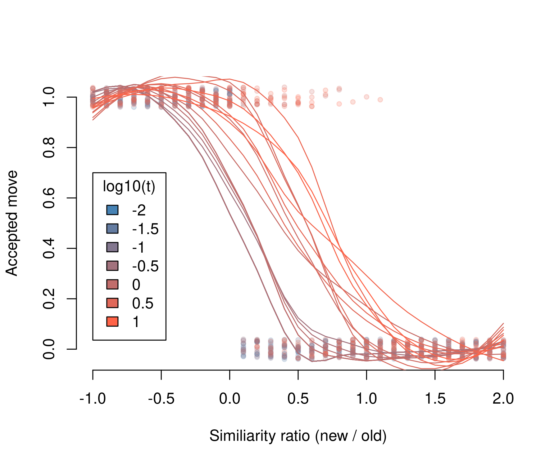
The reason to include this algorithm is to avoid a purely deterministic procedure and include some stochasticity in the process. However, if this is unwanted, it can be removed (and the process made purely deterministic), by specifying a very high temperature parameter t:
table(sapply(seq_len(1000), \(x) metropolis.hastings(1, 1e3, t = 1e9)))
#>
#> TRUE
#> 1000
Similarity trend by move
get_similarity <- function(sp) {
  g <- graph_from_adjacency_matrix(adirondack[sp, sp])
  consumers <- intersect(sp, assembly:::.consumers(adirondack))
  J <- similarity(
    g,
    vids = which(sp %in% consumers)
  )
  diag(J) <- NA
  J <- sum(J, na.rm = TRUE)
  return(J)
}

temps <- 10 ^ seq(-3, 0, by = 1)
sim <- matrix(rep(NA, 300 * length(temps)), ncol = length(temps))
for (t in seq_along(temps)) {
  sp <- sp_resource
  for (i in seq_len(nrow(sim))) {
    sim[i, t] <- get_similarity(sp)
    sp <- assembly:::.move(sp, adirondack, t = temps[t])
  }
}
pal <- colorRampPalette(colors = c("steelblue", "tomato"))(length(temps))
plot(seq_len(nrow(sim)), sim[, 1], frame = FALSE,
     xlab = "Move number", ylab = "Similarity",
     type = "l", col = pal[1], lwd = 2,
     ylim = c(min(sim), max(sim) * 1.25))
for (i in 2:length(temps)) {
  lines(seq_len(nrow(sim)), sim[, i], col = pal[i], lw = 2)
}
legend(x = 70, y = 130, fill = pal, legend = temps,
       title = "Temperature", horiz = TRUE,
       box.lwd = 0, bg = NA)

Verbose output
similarity_filtering() has the options to return verbose output. In
this case, the returned object is not the vector of the name of the
species, but a list with:
- species, the vector with the species names
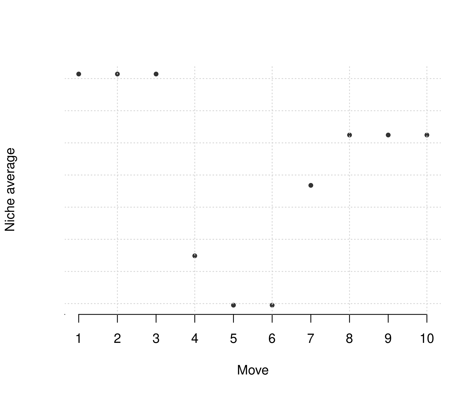
- mean.niche, a vector with containing the mean of the trophic levels of resources for each consumers, averaged over the whole community
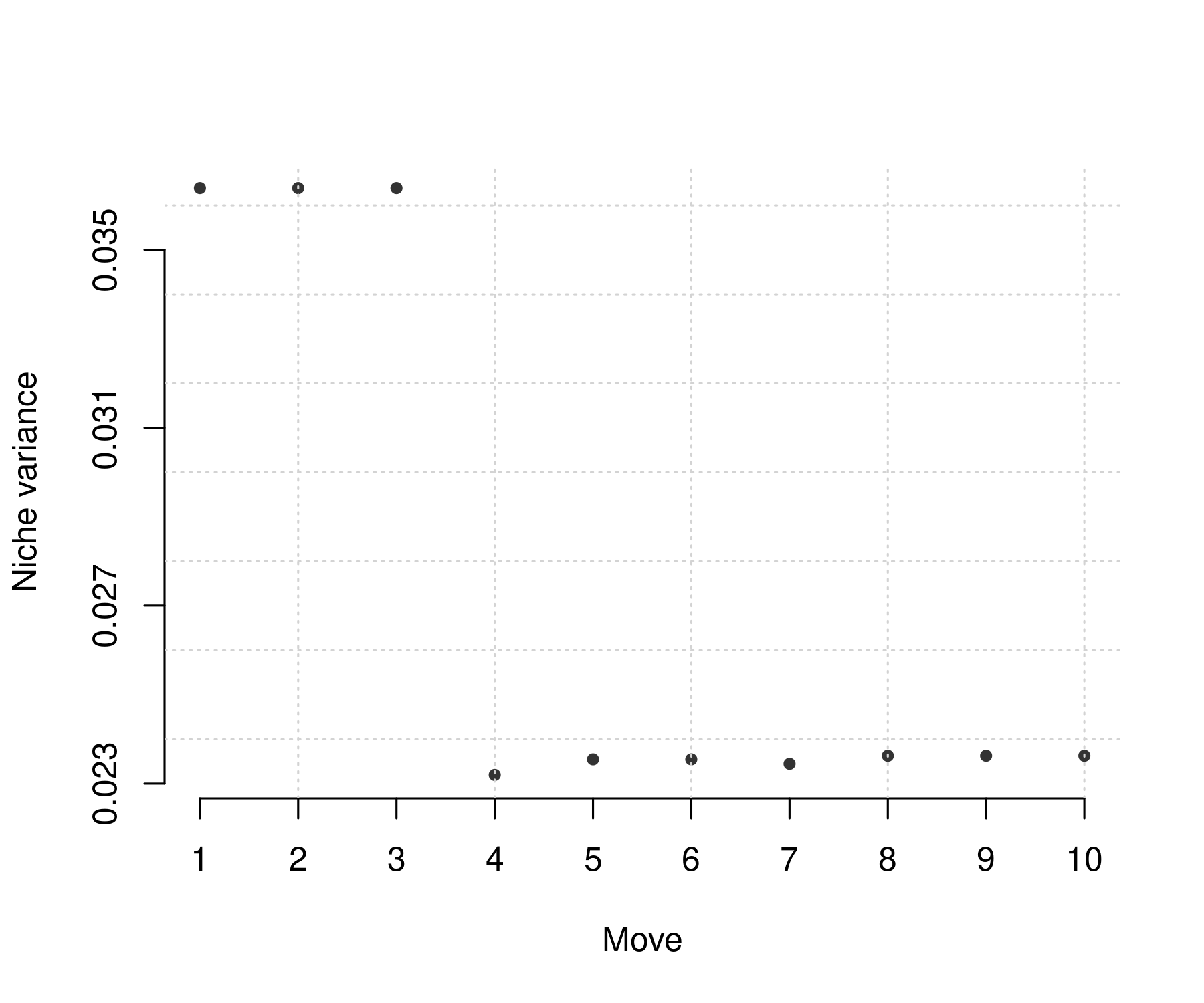
- var.niche, a vector with containing the variance of the trophic levels of resources for each consumers, averaged over the whole community
- similarity the similarity statistics used to evaluate the moves.
Each vector, except species, has length = max.iter. In the case a
move was rejected, the
similarity[i] = 0.
sp_sim <- similarity_filtering(sp_resource, adirondack, t = 1, max.iter = 10,
                               output.verbose = TRUE)
class(sp_sim)
#> [1] "list"
names(sp_sim)
#> [1] "species"    "mean.niche" "var.niche"  "similarity"
This can be useful to check trends in niche packing when species similarity changes. For instance, for increasing similarity, species niche variance should decrease, implying that niches of different species overlap less.
Average niche, however, may change more subtly. For example, decreasing similarity may imply decreasing average niche in the case that lower trophic levels are largely empty. However, it may also imply increasing average niche, e.g. by a new top consumer.
Filtering algorithms and modularity
Jaccard similarity is often used to detect modules in community
detection problems. The rationale is that similarity is high within
modules and low between modules. This implies that the limiting
similarity filtering, in its purely deterministic version
(),
it will converge to food webs that are highly modular, as this minimize
the total Jaccard similarity of the network. This effect is more
pronounced in sparser networks, that is in food webs with lower
connectance.
To illustrate this, I generate 200 random networks for five different connectance levels and calculate the average similarity of the network as well as its modularity metric:
REPS <- 200
CONNECTANCE <- seq(.1, .3, by = .05)

modularity <- matrix(rep(NA, REPS * length(CONNECTANCE)), nrow = REPS)
similarity <- matrix(rep(NA, REPS * length(CONNECTANCE)), nrow = REPS)
for (C in CONNECTANCE) {
  for (rep in seq_len(REPS)) {
    m <- matrix(as.numeric(runif(1e4) < C), 1e2, 1e2)
    g <- graph_from_adjacency_matrix(m)
    members <- membership(cluster_fast_greedy(as.undirected(g)))
    modularity[rep, which (CONNECTANCE == C)] <- modularity(as.undirected(g), members)
    sim <- similarity(g, mode = "in", method = "jaccard")
    similarity[rep, which (CONNECTANCE == C)] <- mean(sim, na.rm = TRUE)
  }
}

Integrating food web dynamics
Until now, we focused on assembly processes and how this influence the topology of the network. It is possible to integrate the assembly with food web dynamics, e.g. comparing dynamics between filtering processes. I collaborated to the ATNr package to solve food web dynamical systems.
Create a synthetic metaweb with virtual species:
library(ATNr)
#>
#> Attaching package: 'ATNr'
#> The following object is masked from 'package:igraph':
#>
#>     is_connected

S <- 200

traits <- data.frame(
  species = sapply(seq_len(S), \(x){
    paste(sample(letters, 10, replace = TRUE), collapse = "")
  }),
  masses = 10 ^ runif(S, 0, 2), #log-uniform
  biomasses = runif(S, 2, 5),
  role = sapply(seq_len(S), \(x) ifelse(runif(1) > .7, "basal", "consumer"))
)

traits <- traits[order(traits$masses), ]

metaweb <- create_Lmatrix(traits$masses,
                          sum(traits$role == "basal"),
                          Ropt = 10,
                          th = .1)
sum(colSums(metaweb) == 0) == sum(traits$role == "basal")
#> [1] TRUE
metaweb[metaweb > 0] <- 1
colnames(metaweb) <- traits$species
rownames(metaweb) <- traits$species
show_fw(colnames(metaweb), metaweb)

Draw random species for a local community of 30 species and impose sequentially the resource filtering and the limiting similarity filtering:
sp <- draw_random_species(30, colnames(metaweb))
length(setdiff(sp, assembly:::.basals(metaweb)))
#> [1] 20
sp_resource <- resource_filtering(sp, metaweb, keep.n.basal = TRUE)
length(setdiff(sp_resource, assembly:::.basals(metaweb)))
#> [1] 20
sp_limiting <- similarity_filtering(sp_resource, metaweb, t = 1e6, max.iter = 1e2)
length(setdiff(sp_limiting, assembly:::.basals(metaweb)))
#> [1] 20

show_graph(sp, metaweb, title = "Random")

show_graph(sp_resource, metaweb, title = "Resource filtering")
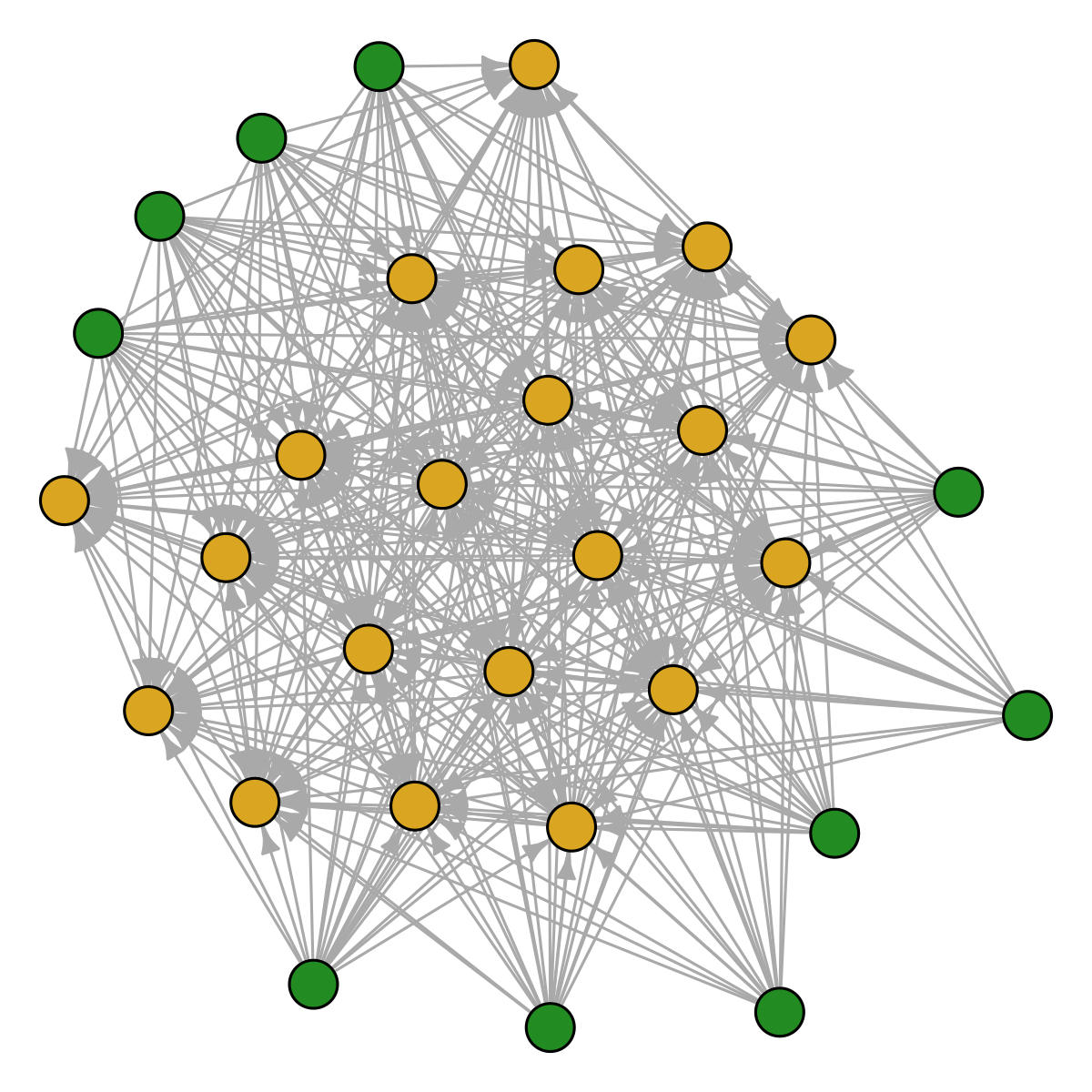
show_graph(sp_limiting, metaweb, title = "Limiting similarity")

Create and initialize the ATNr models:
nb_b <- length(setdiff(sp, assembly:::.basals(metaweb)))
nb_s <- 30

dyn_random <- create_model_Unscaled(nb_s, nb_b,
                                    traits$masses[traits$species %in% sp],
                                    metaweb[sp, sp])
dyn_res <- create_model_Unscaled(nb_s, nb_b,
                                 traits$masses[traits$species %in% sp_resource],
                                 metaweb[sp_resource, sp_resource])
dyn_lim <- create_model_Unscaled(nb_s, nb_b,
                                 traits$masses[traits$species %in% sp_limiting],
                                 metaweb[sp_limiting, sp_limiting])
# default parameters
initialise_default_Unscaled(dyn_random)
#> C++ object <0x55f786c1e9a0> of class 'Unscaled' <0x55f7872708d0>
initialise_default_Unscaled(dyn_res)
#> C++ object <0x55f786a62310> of class 'Unscaled' <0x55f7872708d0>
initialise_default_Unscaled(dyn_lim)
#> C++ object <0x55f78735cf70> of class 'Unscaled' <0x55f7872708d0>
# initialize C++ fields
dyn_random$initialisations()
dyn_res$initialisations()
dyn_lim$initialisations()
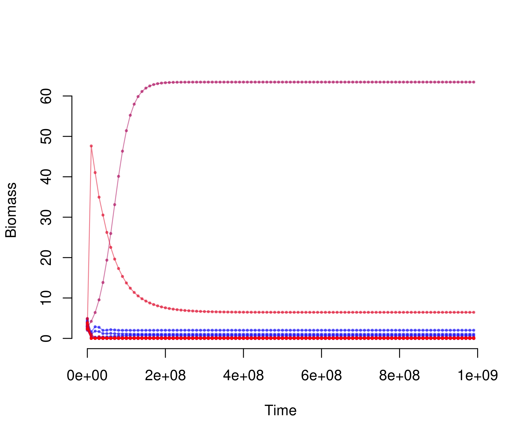
And call the solver to obtain the dynamics:
times <- seq(1, 1e9, 1e7)

sol_random <- lsoda_wrapper(times, traits$biomasses[traits$species %in% sp],
                            dyn_random)
sol_res <- lsoda_wrapper(times, traits$biomasses[traits$species %in% sp_resource],
                         dyn_res)
sol_lim <- lsoda_wrapper(times, traits$biomasses[traits$species %in% sp_limiting],
                         dyn_lim)

plot_odeweb(sol_random, nb_s)
plot_odeweb(sol_res, nb_s)
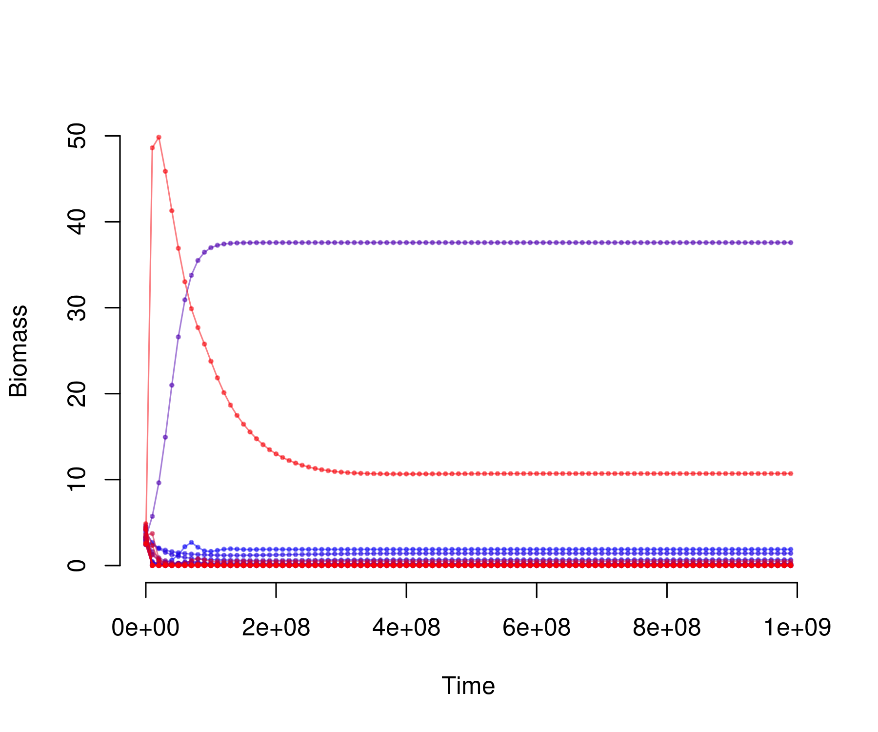
plot_odeweb(sol_lim, nb_s)
The number of extinct species can be extracted by:
sum(sol_random[length(times), -1] < 1e-6)
#> [1] 5
sum(sol_res[length(times), -1] < 1e-6)
#> [1] 5
sum(sol_lim[length(times), -1] < 1e-6)
#> [1] 0
As well as the final total biomass of all consumers combined:
sum(sol_random[length(times), (nb_b + 2) : nb_s])
#> [1] 11.45064
sum(sol_res[length(times), (nb_b + 2) : nb_s])
#> [1] 11.45064
sum(sol_lim[length(times), (nb_b + 2) : nb_s])
#> [1] 7.290431